Research Projects


Topological Solitons: The Skyrme Model in 2+1 dimensions (babyskyrmions)

What doth thy skyrmion out of his bed at midnight? Shall I give him his answer?
inspired from Shakespeare, Henry IV, part 1, Act 2, Scene 4     Skyrmion newsskyrme_newshtml.


head-on collision at γ=2.29 Click me to watch the animation 39  4454

Skyrmions are topological soliton solutions of a classical nonlinear field theory known as the Skyrme model. As examples of two and three-dimensional solitonic structures, they are of inherent interest, but they may also have applications to nuclear physics. The Skyrme model can be obtained as a low energy limit of QCD in the large Nc limit (Nc the number of colours), with baryons being identified as quantized states of the classical soliton solutions. QCD is very difficult to solve in the strong coupling regime (low energy), even numerically. Interest turned to simpler phenomenological models for the structure of hadrons. The Skyrme model in 2+1 dimensions is know as the baby skyrme model. These nonlinear σ-models in 2+1 appear to be low dimensional analogues to four-dimensional Yang-Mills theories.

Left we can see the different stages of a head-on collision of two babyskyrmions in the plane. We observe the Baryon number density profiles of each soliton. The initial data is boosted to γ=2.29; (v=0.9c). We can see that they scatter at right angles. This is very typical for solitons of wave-like equations.

As a numerical relativist this model represents an ideal testbed for numerical techniques, since the numerical integration of the Skyrmion field equations is technically similar to that found with Einstein Equations. Another motivation is the possibility to use skyrmions as another type of source matter, along with scalar fields and fluids. Coupling a skyrmion matter lagrangian to Einstein equations leads to interesting bound states in curved space-time. Another possibility is to use a skyrmion equation fo state to integrate the Tolman-Oppenheimmer-Volkoff equations to study star-like solutions.

I am interested in the dynamics of highly boosted collisions of skyrmions, since one of the most most interesting and challenging aspects of the Skyrme model constitutes the numerical instabilities reported for large velocities. It has been suggested that the hyperbolic nature of the equations is lost, turning the problem ill-posed  I have performed extensive 2+1 and 3+1 simulations of skyrmion collisions at high boosts (γ ~ 10) using parallel adaptive mesh refinement techniques (PAMR). It has been shown that causality is not violated in the Skyrme model, so the idea is to determine if the instabilities araise from inadequate numerical methods, or they have a physical origin.

Understanding of skyrmion scattering and dynamics  is also proving to be fruitful in dense hadronic matter relevant to compact stars, a system difficult to access by other approaches. The recent discovery of holograFc baryons in gravity/gauge duality which correspond to skyrmions in the infinite tower of vector mesons provides a window to the regime of strong coupling, that QCD proper has difficulty in accessing. Interest on topological solitons is manifold. They also provide models for matter at high energies and velocities. A numerical understanding of collisions of ultra-relativistic solitons in the presence of gravity  may shred light  on many issues at the crossroads of space-time singularity formation, heavy-ion dynamics and exotic new physics in extra-dimensions, where black-holes are expected to form in the next generation of Tera-Scale energy accelerators.


Topological Solitons: The Skyrme Model in 3+1 dimensions


Comming soon

Non-topological Solitons: Q-balls in 2+1 and 3+1 dimensions

qball
qball
In 3 spatial dimensions we simply solve a different equation for the initial data (one involving the 3d laplacian operator) and we obtain a static solution, but in this case we have to take slices (for example the one above) of the 3d Q-ball setup (cube below) and observe the time evolution. Since the real and imaginary parts of the complex scalar field of a Q-ball are a cosine and a sine respectively, we visualize the |Φ| modulus of the complex scalar field, where the localized nature of the soliton can be appreciated.
qball3d cube
It is well known that realistic supersymmetric theories are associated with a number of scalar fields with various charges, which allow for baryonic and leptonic non-topological solitons known as Q-Balls.  A Q-Ball is a solution of a relativistic (complex) scalar field theory with a non-linear quadratic potential, which depends on the supersymmetry breaking mechanism, and there is a conserved Noether charge Q carried by the Q-Ball lump. We can also have spinning Q-Balls, which carry angular momentum. 
The basic properties of Q-Balls are well understood using analytical methods, for example existence and  stability under small vibrations. I intend to continue my work on numerical simulations of Q-Ball evolution in 2+1 (two spatial dimensions and time) and 3+1 dimensions to address strong coupling dynamics such as  scattering, interactions and stability, and to perform a parameter space exploration using PAMR techniques. Is there any exotic scattering? right-angle scattering for topological solitons depends on the velocity of the impact, do nontopological solitons, such as Q-Balls, exhibit the same behaviour?  A detailed knowledge of Q-ball scattering is needed to answer several questions in cosmology,  where they could be responsible for both the net baryon number of the universe and its dark matter component. Q-Balls may be trapped in neutron star interiors. So far this questions are being addressed in Flat space time. I would like to explore the possibility to search for self-gravitating Q-balls.

Ultra-relativistic Head-on-Collision video
skyrmionskyrmion skyrmionskyrmion
Video and snapshots of the head-on collision of two qballs in 2+1 dimensions with the same phase ω. We show the |Φ| modulus of the complex scalar field of the q-balls. The initial data is boosted to γ=7.08 (v=0.99c).We can see the interference pattern at the center of the colission, since the evolution equation is wave-like. Notice the Lorentz contraction in the q-ball profiles.

I am using q-balls as a model for matter in ultra-relativistic collisions. This regime has not been exhaustively explored and it is my intention to do so. Highly boosted matter is challenging since higher resolutio is needed and instabilities are more likely to appear. There are other types of matter that show unexpected and rich behaviour at high velocities, such as skyrmions. Other objects of interest based on a complex scalar field are boson stars. The difference is that they incorporate a quadratic potential, and naturally gravity is included in the lagrangian so the competition between the collapse and the scalar field "pressure" outwards reach an equilibrium configuration that we call a star. My collegue Bruno Mundim has studied those objects intensively.


Topological Solitons: The Skyrme Model in 2+1 dimensions stabilized by vector mesons


Kinks, Domain Walls and branes


The video in the right shows the collision of a kink and an antikink of a φ^4 field theory in 1+1 dimensions, at low velocity (v=0.3c). This relatively simple setup can be used to model the 3+1 boundary (a brane) of a 4+1 bulk, given certain symmetry assumptions.  Fermions become localized since they tend to stick to the kink defect rather than escaping as radiation to the bulk. The kink in the scalar field acts as an impurity that traps the fermion on the brane, similarly to some condensed matter systems where a magnetic field provides the "impurity". This trapping is analogous to the requirement that fermions must live on the brane. The particle number (fermion content) on moving kinks changes after a kink-antikink collision, or when these 1+1 "domain walls" collide with the spacetime boundaries, and we can compute this particle transfer calculating Bogoliubov (transmission-reflection) coefficients. Pionnering work in this direction has been performed by Gibbons, Maeda and Takamizu, and subsecuently by   Saffin and Tranberg . These toy models for fermions on colliding branes represent a very instructive effort to understand more realistic braneworld scenarios. My idea is to extend the kink collisions code I have to incorporate mesh refinement. It may also be interesting to study highly boosted kink-antikink collisions in this framework. I would like to test convergence and conserved quantities and extend all this interesting work, which constitutes one more example of the very healthy interplay between condensed matter, high energy theory and numerical analysis.
kink-antikink collision 0.3c


Constrained Evolution and Constraint Damping


Particle-Particle and Particle Mesh Methods with PAMR


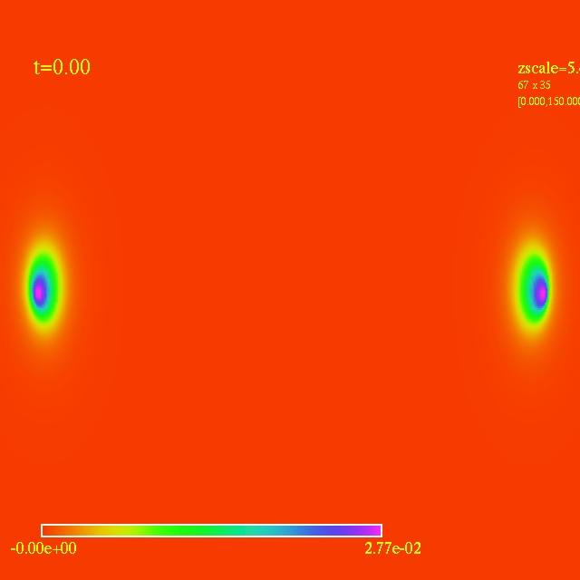
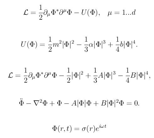
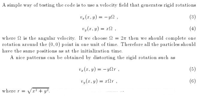
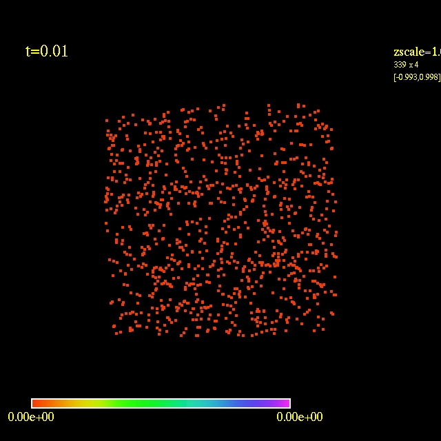
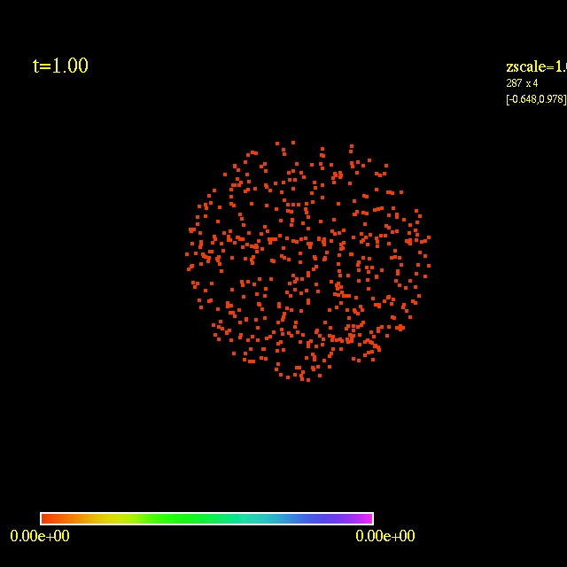
Left: initial configuration; Right: end configuration with the analytic velocity  field independent of the radius.


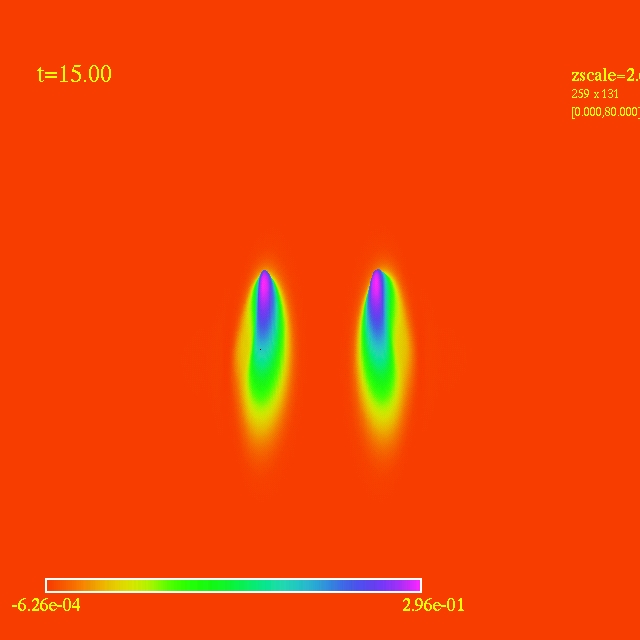
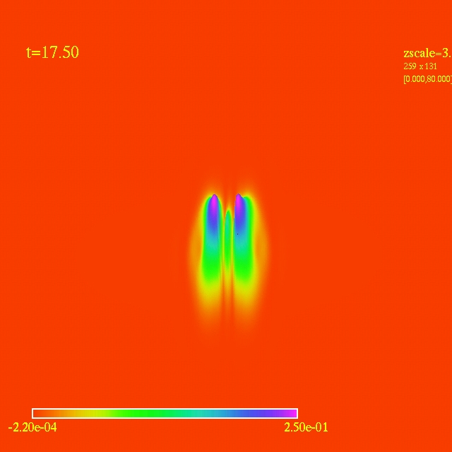
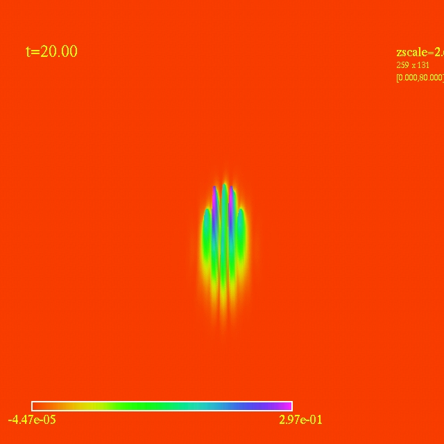
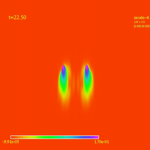
  • Here I have some movies of the evolutions: (120 steps each)
    movie processors Nparticles vtype resolution
    movie1.mpg 4 1000 1 256x256
    movie2.mpg 4 1000 1 640x640
    movie3.mpg 8 1000 1 640x640
    movie4.mpg 8 1000 2 640x640
    movie5.mpg 16 1000 2 640x640
    movie6.mpg 3 1000 3 640x640


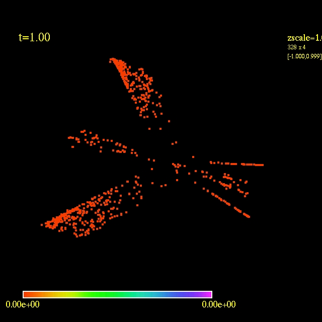
    In this video the velocity components of each of the 3000 particles in the configuration depends as vx=sin(py/px) and vy=cos(py/px), where px and py are the x and y positions of each particle respectively. They exit the domain in Jet-like patterns.


This is a parallel application to simulate the motion of test particles in a given velocity field, for instance, the motion of smoke particles in the wind. Consider a 2D domain. The parallelization  and  domain decomposition are done by PAMR, each processor evolves the particles that currently belong to its subdomain. Particles migrate from subdomain to subdomain and also leave the domain completely. This approach is efficient as long as the particles are approximately uniformly distributed over the domain.

The domain is a square with the left lower corner at (-1, -1) with its center at (0, 0). We can evaluate the velocity field at each point of the domain analitically , i.e., we know the functions vx (x, y) and vy (x, y).  I use a  second order Runge-Kutta scheme to advance each particle position from time level n to time level n + 1 by Δt,

Runge-Kutta scheme
Rotational Velocity Field


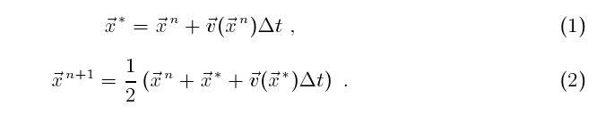
The next step is to migrate particles that leave a processor's subdomain into the corresponding  new one. The way  implemented here is that each processor broadcasts the positions of particles that left its subdomain. Each processor then selects the particles belonging to its subdomain. Note that in general the domain is
not filled with particles uniformly, so that processors must handle different number of them at a given time.
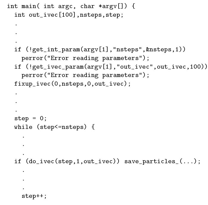
The bbhutils offer an easy way for reading parameters from files, Especially useful is the ivec type. The ivec type allows for easy and compact notation of specifying an index vector. This is useful for output control. The next snippet of code shows how to use the variable out ivec to control the output frequency. The parameter file is passed as the first command line argument.

read.jpg  

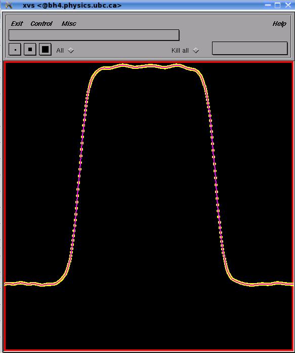
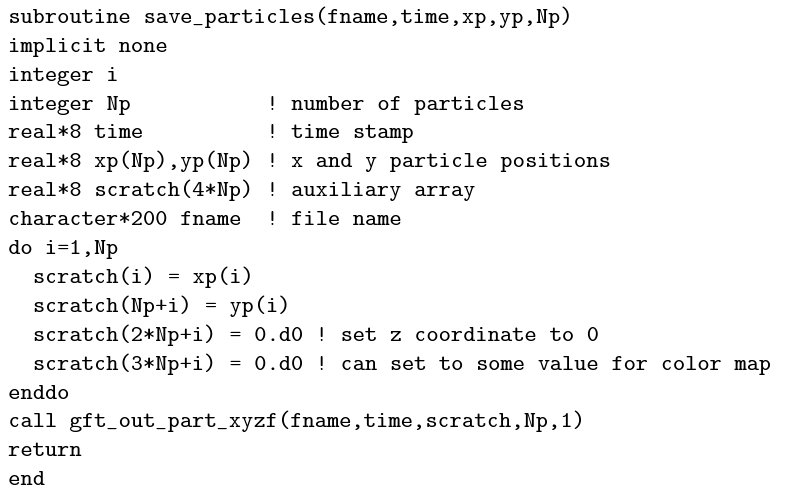
The data can be viewed by DV by selecting the item Particles from the options menu of the DV local view window. The following is an example of a C routine that saves a 2D particle data:

Save Particles
The particle positions are initialized randomly generating particles
within a desired domain.

Randome Initialization of positions


Source Code
  • The code consists in a main.c program written in C, that uses PAMR calls and standard MPI calls. The file fortran.f contains the subroutines initialize, save_particles and make_step. As a template i used on of Martins examples of the course, one of the unigrid codes.
  • The number of particles in each subdomain is the same, Np; PAMR 
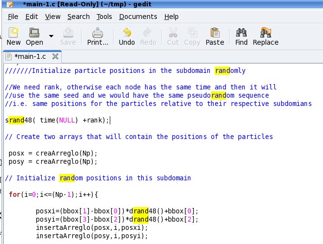
performs the subdivision. The particles are initialized randomly. I need the rank, otherwise each node has the same time and then it will use the same seed and we would have the same pseudorandom sequence i.e. same positions for the particles relative to their respective subdomains srand48( time(NULL) +rank);
  • The make_step subroutine is written in fortran, along with a bunch of other subroutines found in the same file fortran.f
  • the parameter file id provides the type of velocity field to be used, the number of particles and the number of time steps to be performed. The actual time step length is defined inside the program.

  • I checked the subdivision looking at the bbox vertices when I started to write the program.
  • As requested, the vtype variable indicates which type of velocity is used: 1) analytic field independent of r, 2) analytic field dependent of r, 3) grid velocity field; where r is the radius of the particle with respect to the center.
Grid Velocity Field
  • Instead of  a known analytic velocity field,  the velocity can be defined only on a grid. The simplest model is a time independent the velocity field.  The velocity at any given point use linear interpolation using the four vertices that surround a given point, first interpolating in the x-direction and then in the y-direction. Two ghost zones are employed for buffering. Note that the time step  should be sufficiently small so that a particle from inside the domain does not migrate beyond the buffer zone in the first Euler substep (1) (so we can complete the Runge-Kutta step). This model can be used to visualize fluid flows that are calculated on a computational grid (of course in that case the velocity field would be also time dependent). The higher the resolution  of the the grid the closer the results should be to the analytic profile. 
  • The grid velocity field is implemented: I made sure particles dont make a large first RK step so they go out of the ghost cells (I use two), so the program can calculate the velocity for the second RK step; in main.c I set up a grid velocity field using two arrays. I populate vx and vy on the grid using the analytical field independent of r (of course the grid can store arbitrary values of vx and vy). I was not able to use PAMR completely for this matter. So I created the grid manually using arrays and then I pass it to the make_step fortran subrotuine; then the velocity is interpolated from the grid values and calculated at any arbitrary point of the subdomain. This still needs work to do.


Architecture of the code
  • The total number of particles NT is divided by the number of processors p; PAMR subdivides the domain in p subdomains each with Np particles and the positions are initialized randomly.
  • A set of array-like data structures are defined to deal with dynamic arrays in an easy way (for me). I began using these data structures but they turned out not to be very flexible in some situations so they appear mixed with ordinary dynamical arrays.
  • We start the evolution: we create arrays posx and posy to store the positions of the particles of each subdomain; we save the particle positions here to sdf files.
  • The particle positions are evolved using a Runge-Kutta second order scheme as requested; if the particle does not belong to the domain any more it is placed in two migration arrays mx,my; posx and posy are shrinked to a new size (creating and destroying arrays dynamically).
  • Given the fact that the sizes of mx,my are different for each processor, I designate a master processor (the rank=0 cpu) so it uses a MPI_Gather call to gather all the sizes of the migration arrays from each processor; the sum of all sizes is totalN, so the master processor creates recvArrayx and recvArrayy to allocate the migrants positions.
  • The master processor uses two MPI_Gatherv calls to gather the x and y positions of all migrants from all processors and populate recvArrayx and recvArrayy.
  • The migrants arrays are broadcasted to all processors; in order for them to allocate the migrants positions, totalN is broadcasted to all processors so each creates two arrays for the "newcomers".
  • We advance t=t+dt;
  • Each processor takes those migrants which belong to its subdomain; then each node merges the newcomers with those particles already in the domain and we obtain the new posx and posy arrays; we save them to sdf and we make the next runge-kutta step
  • The process is repeated N time steps. All this involves the creation, resizing and destruction of lots of arrays.


Compiling and Running the program
  • My Makefile
  • The process is the usual:
    1 cd 2d
    2 make clean
    3 source /home3/vnfe4/home/benjamin/2d/soPGI-mpich
    4 make
  • id is the parameter file:
  • mpirun -np 3 -machinefile machfile par2d.exe id

Scaling

I set the analytic velocity field so the particles go in circles; 1=N*dt where N is the number of time steps and dt is the time-length of the time step; the local error or a Runge-Kutta scheme of second order is supossed to be proportional to dt^3, and the global error proportional to dt^2; I was not sure about this and I decided to write a program that would evolve a complete orbit of a single particle located at radius=1 using this scheme; then i calculated the error of the radius after the orbit and the relative error dr/r for different values of dt and N time steps such that N*dt=1; the results are shown in this file and the following graph. Starting from N=27 and dt=0.037, the relative error is ~1%, so if we use a dt=0.01 and 100 or so time steps, we are safely well below 1 percent of relative error in the radius after one orbit.

  •  


  • So for the Scaling of the code I constructed the following table (the times are measured in seconds using MPI_Wtime):

    Total Number Particles 2 processors 4 6 8 16
    100 0.027017 0.461920 0.494730 0.67247 1.202543
    1000 1.820399 1.888175 1.773452 1.981796 2.006310
    10000 14.319587 8.407474 6.911991 7.149420 13.688003
    100000 340.282804 286.478503 289.795620 287.918076 728.096616


    We can appreciate theese results in the following log-log plot:
  • Theoretically, Linear speedup or ideal speedup is obtained when it is equal to the number of processors. When running an algorithm with linear speedup, doubling the number of processors doubles the speed. As this is ideal, it is considered very good scalability.
  • As we know intercommunication latency and other factors, such as the speed of memory, I/O operations, etc. reduce the speedup.
  • We can see from the graph that for 100 particles the time grows very fast when N is increased; for a small number of particles the scaling is very bad; for 1000 particles it does not change much; for 10,000 and 100,000 particles the execution time seems to decrease and then it reverts to the original trend.
  • It looks like scaling is more efficient for a large number of particles rather than for a few.


  • Preprints of Interest


    skyrmion


    Fri Apr 22 02:39:13 PDT 2011