Singularities

Before exploring the behavior of test particles in the Schwarzschild spacetime, allow us to say a word about singularities. From the form of (1), the metric coefficients become infinite at $r = 0$ and $r = 2GM$, an apparent sign that something is going wrong. The metric coefficients, of course, are coordinate-dependent quantities, and as such we should not make too much of their values; it is certainly possible to have a "coordinate singularity" which results from a breakdown of a specific coordinate system rather than the underlying manifold. An example occurs at the origin of polar coordinates in the plane, where the metric is $ds^2=dr^2+r^2d\theta^2$ becomes degenerate and the component $g^{\theta\theta}=r^{-2}$ of the inverse metric blows up, even though that point of the manifold is no different from any other.

What kind of coordinate-independent signal should we look for as a warning that something about the geometry is out of control? This turns out to be a difficult question to answer, and entire books have been written about the nature of singularities in general relativity. We won't go into this issue in detail, but rather turn to one simple criterion for when something has gone wrong - when the curvature becomes infinite. The curvature is measured by the Riemann tensor, and it is hard to say when a tensor becomes infinite, since its components are coordinate-dependent. But from the curvature we can construct various scalar quantities, and since scalars are coordinate-independent it will be meaningful to say that they become infinite. This simplest such scalar is the Ricci scalar $R = g^{\mu\nu} R_{\mu\nu}$, but we can also construct higher-order scalars such as $R^{\mu\nu}R_{\mu\nu}$, $R^{\mu\nu\rho\sigma}R_{\mu\nu\rho\sigma}$, $R_{\mu\nu\rho\sigma}R^{\rho\sigma\lambda\tau}R_{\lambda\tau}^{\mu\nu}$ and so on. If any of these scalars (not necessarily all of them) go to infinity as we approach some point, we will regard that point as a singularity of the curvature. We should also check that the point is not "infinitely far away"; that is, that it can be reached by travelling a finite distance along a curve.

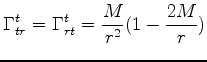
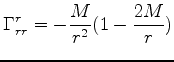
We therefore have a sufficient condition for a point to be considered a singularity. It is not a necessary condition, however, and it is generally harder to show that a given point is nonsingular; for our purposes we will simply test to see if geodesics are well-behaved at the point in question, and if so then we will consider the point nonsingular. In the case of the Schwarzschild metric (1), direct calculation reveals that

$$R^{\mu\nu\rho\sigma}R_{\mu\nu\rho\sigma}= \frac{12G^2M^2}{r^6}$$ (2)

This is enough to convince us that r = 0 represents an honest singularity. At the other trouble spot, $r = 2GM$ , you could check and see that none of the curvature invariants blows up. We therefore begin to think that it is actually not singular, and we have simply chosen a bad coordinate system. The best thing to do is to transform to more appropriate coordinates if possible. We will soon see that in this case it is in fact possible, and the surface $r = 2GM$ is very well-behaved (although interesting) in the Schwarzschild metric.

Having worried a little about singularities, we should point out that the behavior of Schwarzschild at $r\leq 2GM$ is of little day-to-day consequence. The solution we derived is valid only in vacuum, and we expect it to hold outside a spherical body such as a star. However, in the case of the Sun we are dealing with a body which extends to a radius of

$$R_\odot = 10^6 GM_\odot$$ (3)

Thus, $r = 2GM_\odot$ is far inside the solar interior, where we do not expect the Schwarzschild metric to apply. In fact, realistic stellar interior solutions consist of matching the exterior Schwarzschild metric to an interior metric which is perfectly smooth at the origin. See Schutz for details. Nevertheless, there are objects for which the full Schwarzschild metric is required - black holes - and therefore we will let our imaginations roam far outside the solar system in this section.

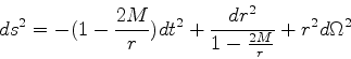
From now on we will consider geometrized units, i.e. $G=c=1$, so our metric takes the form,

$$ds^2 = -(1-\frac{2M}{r})dt^2+\frac{dr^2}{1-\frac{2M}{r}}+r^2 d\Omega^2$$ (4)

The first step we will take to understand this metric more fully is to consider the behavior of geodesics. We need the nonzero Christoffel symbols for Schwarzschild. We calculated them using Maple and GRTensor:

$$\Gamma^t_{tr}=\Gamma^t_{rt}=\frac{M}{r^2}(1-\frac{2M}{r}) \Gamma^r_{tt}=\frac{M}{r^2}(1-\frac{2M}{r}) \Gamma^r_{rr}=-\frac{M}{r^2}(1-\frac{2M}{r})$$

$$\Gamma^r_{\theta\theta}=-r(1-\frac{2M}{r}) \Gamma^r_{\phi\phi}=-r sin^2(\theta)(1-\frac{2M}{r}) \Gamma^\theta_{r\theta}=\Gamma^\theta_{\theta r}=\frac{1}{r}$$

$$\Gamma^\theta_{\phi\phi}=-sin(\theta)cos(\theta) \Gamma^\phi_{r\theta}=\Gamma^\phi_{\theta r}=\frac{1}{r} \Gamma^\phi_{\theta\phi}=\Gamma^\phi_{\phi\theta}=cot(\theta)$$

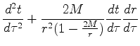
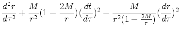
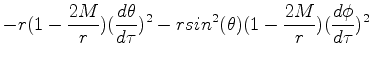
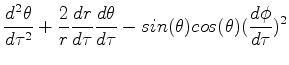
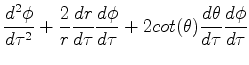
The geodesic equation follows from a variational principle, and we will talk about it later. Now we will just use

$$\frac{d^2x^\alpha}{d\tau^2}+\Gamma^{\alpha}_{\beta\gamma}\frac{dx^\beta}{d\tau}\frac{dx^x\gamma}{d\tau}$$ (5)

which turns into the following four equations, using spherical coordinates where $\tau$ is an affine parameter²:

$$\frac{d^2t}{d\tau^2}+\frac{2M}{r^2(1-\frac{2M}{r})}\frac{dt}{d\tau}\frac{dr}{d\tau} = 0$$

$$\frac{d^2r}{d\tau^2}+\frac{M}{r^2}(1-\frac{2M}{r})(\frac{dt}{d\tau})^{2}-\frac{M}{r^2(1-\frac{2M}{r})} (\frac{dr}{d\tau})^2$$

$$-r(1-\frac{2M}{r})(\frac{d\theta}{d\tau})^2-rsin^2(\theta)(1-\frac{2M}{r})(\frac{d\phi}{d\tau})^2 = 0$$

$$\frac{d^2\theta}{d\tau^2}+\frac{2}{r}\frac{dr}{d\tau}\frac{d\theta}{d\tau}-sin(\theta)cos(\theta)(\frac{d\phi}{d\tau})^2 = 0$$

$$\frac{d^2\phi}{d\tau^2}+\frac{2}{r}\frac{dr}{d\tau}\frac{d\phi}{d\tau}+2cot(\theta)\frac{d\theta}{d\tau}\frac{d\phi}{d\tau} = 0$$

Now we will proceed to analyze our equations using the symmetries of the Schwarzschild metric. These symmetries will also be usefull when we implement our code. There are four killing vectors: three of the spherical symmetry and one for time translations (our metric is static). Each of them lead to a constant of motion for a free particle; if $K^{\mu}$ is a killing vector, we know that:

$$K_{\mu} = \frac{dx^\mu}{d\tau}$$ (6)

We also have another constant of motion always present for geodesics; metric compatibility implies that along the path the quantity,

$$\epsilon = -g_{\mu\nu}\frac{dx^\mu}{d\tau}\frac{dx^\nu}{d\tau}$$ (7)

is constant. For a massive particle we choose $\tau$ as the proper time of the particle. Then this relation simply becomes $\epsilon = -g_{\mu\nu}U^\mu U^\nu =+1$. For a massless particle (null geodesics) we would have $\epsilon = 0$ , and finally $\epsilon=-1$ corresponds to spacelike geodesics, but they do not correspond to paths of particles. In this homework we are basically concerned with massive particles.

Rather than immediately writing out explicit expressions for the four conservedquantities associated with Killing vectors, let's think about what they are telling us. Notice that the symmetries they represent are also present in flat spacetime, where the conserved quantities they lead to are very familiar. Invarianceunder time translations leads to conservation of energy, while invariance underspatial rotations leads to conservation of the three components of angular momentum. Essentially the same applies to the Schwarzschild metric. We can think of the angular momentum as a three-vector with a magnitude (one component) and direction (two components). Conservation of the direction of angular momentum means that the particle will move in a plane. We can choose this to be the equatorial plane of our coordinate system; if the particle is not in this plane, we can rotate coordinates until it is. Thus, the two Killing vectors which lead to conservation of the direction of angular momentum imply

$$\theta=\frac{\pi}{2}$$ (8)

The two remaining Killing vectors correspond to energy and the magnitude of angular momentum. The energy arisesfrom the timelike Killing vector $K = \partial_t$, or

$$K_\mu = (-(1-\frac{2M}{r},0,0,0))$$ (9)

The Killing vector whose conserved quantity is the magnitude of the angular momentum is $L = \partial_\phi$, or

$$L_\mu = (0,0,0,r^2 sin^2\theta)$$ (10)

Since (8) implies that $sin\theta=1$ along the geodesics we are interested in, the two conserved quantities are

$$E=(1-\frac{2M}{r})\frac{dt}{d\tau}\hspace{0.5cm}and\hspace{0.5cm}L= r^2\frac{d\phi}{d\tau}$$ (11)

If we consider massive particles, hey represent the energy and and angular momentum per unit mass; for massles particles these can be tought of as the energy and angular momentum. The second equation is the GR analog to Kepler's second law (equal areas are swept at equal times).

The set of quantities 11 provide a convenient wat to understand the orbits of particles in the Schwarzschild spacetime. Expanding the expression for $\epsilon$ in (7) we have,

$$-(1-\frac{2M}{r})(\frac{dt}{d\tau})^2+-(1-\frac{2M}{r})^{-1}(\frac{dr}{d\tau})^2+r^2(\frac{d\phi}{d\tau}^2)=-\epsilon$$ (12)

Multiplying this equation by $(1-\frac{2M}{r})$ and using the expressions $(\ref{cons})$ for E and L, we get

$$-E^2+(\frac{dr}{d\tau})^2+(1-\frac{2M}{r})(\frac{L^2}{r^2}+\epsilon)=0$$ (13)

We got a single equation for $r$ in function of $\tau$. We can rewrite it as:

$$\frac{1}{2}(\frac{dr}{d\tau})^2+V(r)=\frac{1}{2}E^2$$ (14)

where

$$V(r)=\frac{1}{2}\epsilon-\epsilon\frac{M}{r}+\frac{L^2}{2r^2}-\frac{ML^2}{r^3}$$ (15)

We are going to plug back the original units of this expression,

$$V(r)=\frac{1}{2}\epsilon-\epsilon\frac{GM}{r}+\frac{L^2}{2r^2}-\frac{GML^2}{r^3}$$ (16)

Doing so we can see that (14)this looks like the equation of a classical particle of unit mass and ``energy'' $\frac{1}{2}E^2$ moving ina one dimensional potential given by $V(r)$³. Plotting the potential provides in sight in the nature of the geodesics. Two plots are shown in figure (1), ilustrating the Newtonian and the Gr behavior of the potential.

Figure 1: Effective ``potential'' for different values or $L$ used to analize the nature of geodesics, for the Newtonian and GR cases.

Of course, our physical situation is quite different from a classical particle m oving in one dimension. The trajectories under consideration are orbits around a star or other object. The quantities of interest to us are not only $r(\tau)$, but also $t(\tau )$ and $\phi(\tau)$. Nevertheless, we can go a long way toward understanding all of the orbits by understanding their radial behavior, and it is a great help to reduce this behavior to a problem we know how to solve.

A similar analysis of orbits in Newtonian gravity would have produced a similar result; the general equation (14) would have been the same, but the effective potential (16) would not have had the last term. (Note that this equation is not a power series in $1/r$, it is exact.) In the potential (16) the first term i s just a constant, the second term corresponds exactly to the Newtonian gravitat ional potential, and the third term is a contribution from angular momentum whic h takes the same form in Newtonian gravity and general relativity. The last term , the GR contribution, will turn out to make a great deal of difference, especia lly at small r.

For Newtonian gravity and $L\neq 0$, $V\rightarrow +\infty$ as $r\rightarrow 0$. Massive particles can approach the star/planet, and disappear to infinity like a comet. Or they can be caught in circular or ellipsoidal orbits. Massless particles travel in straight lines and never stay near the object.

For general relativity and $L\neq 0$, $V(r) \rightarrow -\infty$ as $r\rightarrow 0$. This indicates that massive and massless particles very close to the center r = 0 cannot escape anymore. This is the signal of the horizon of the black hole. Massive particles can follow comet-like trajectories, circular orbits that can be stable or unstable, and more or less ellipsoidal orbits that are not quite ellipsoidal. Photons can also travel in unstable circular orbits.

Let us examine the kinds of possible orbits, as illustrated in the figures. There are different curves $V(r)$ for different values of L; for any one of these curves, the behavior of the orbit can be judged by comparing the $\frac{1}{2}E^2$ to $V(r)$. The general behavior of the particle will be to move in the potential until it reaches a "turning point" where $V (r)=\frac{1}{2}E^2$ where it will begin moving in the other direction. Sometimes there may be no turning point to hit, in which case the particle just keeps going. In other cases the particle may simply move in a circular orbit at radius $r_c = const$; this can happen if the potential is flat, $dV/dr = 0$. Differentiating (16), we find that the circular orbits occur when

$$\epsilon GMr^2_c-L^2r_c+3GML^2\gamma=0$$ (17)

where we introduced the parameter $\gamma$ to appreciate the GR and Newtonian limits in a practical way, so $\gamma=0$ in Newtonian gravity and $\gamma=1$ in general relativity. Circular orbits will be stable if they correspond to a minimum of the potential, and unstable if they correspond to a maximum. Bound orbits which are not circular will oscillate around the radius of the stable circular orbit.

For massless particles, this means $r_0 = 3\gamma GM$ . Thus, in Newton theory photons never travel on circular orbits, in general relativity they can, the orbits are always unstable though and $r_0 = 3GM$ , which is $3/2$ times the Schwarzschild radius.

For massive particles,

$$r_0 = frac{L^2\pm\sqrt{L^4-12(GM)^2\gamma L^2}}{2GM}$$ (18)

So in Newton theory there is always a stable circular orbit for $r_0 = \frac{L^2}{GM}$. For general relativity there are no circular orbits for $L^2 \leq 12(GM )^2$, there is one at $r_0 = 6GM$ for $L^2 = 12(GM )^2$, and there are two for L2 ? 12(GM )2, an unstable one at $r_0 = r_{-}$ and a stable one at $r_0 = r_{+}$. The latter is the one that approaches the Newtonian one as L becomes large. The orbit at $r_0 = r_{-}$ approaches the photon orbit at large $L$, $r_{-} \rightarrow 3GM$ as $L \rightarrow 1$. We have therefore found that the Schwarzschild solution possesses stable circula r orbits for $r > 6GM$ and unstable circular orbits for $3GM < r < 6GM$ . It's important to remember that these are only the geodesics; there is nothing to stop an accelerating particle from dipping below $r = 3GM$ and emerging, as long as it stays beyond $r = 2GM$.