Initial Parameters and Space-times

In order to solve the system we must have 8 initial parameters. Namely, $x^\alpha$ and $\dot{x}^\alpha$. With no loss of generality we will fix $t_0 = 0$ and $\dot{t}$.

$$\dot{t}_0 = \sqrt{(1.0+g_{22}{\dot{r}_0}^2+g_{33}{\dot{\theta}_0}^2+g_{44}{\dot{\phi}_0}^2)/(-g_{11})}$$ (6)

where,

$$\dot{f}=\frac{df}{d\tau}$$

The rest may be freely specified. During our experimentation we started at the most obvious place, Schwarzschild. Because of the t independence it greatly simplified things and we were able to test and debug properly. Also, it provided some very nice looking solutions.

Schwarzschild Metric

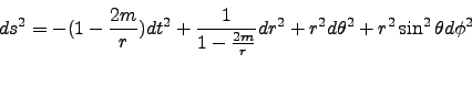$$ds^2 = -(1-\frac{2m}{r})dt^2 + \frac{1}{1-\frac{2m}{r}}dr^2 + r^2 d\theta^2 + r^2 \sin^2{\theta} d\phi^2 \vspace{1cm}$$ (7)

3-sphere in a 4-dimensional cartesian space

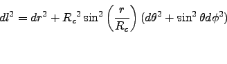$$dl^2 = dr^2 + {R_c}^2 \sin^2\left(\frac{r}{R_c}\right) (d\theta^2 + \sin^2\theta d\phi^2 ) \vspace{1cm}$$ (8)

homogeneous 3-space

$$dl^2 = dr^2 + {R_c}^2 \sinh^2\left(\frac{r}{R_c}\right) (d\theta^2 + \sin^2\theta d\phi^2 )$$ (9)