The Routine

A perlTk script drives the full procedure. We used perlTk because of its ease to program, Ben was familiar with it and is easy of use. The only downside is that it requires interpretation. In the future we are planning to implement in java so as to allow more portability.

The perl script calls maple with a pre-programmed routine to create a subroutine that would provide us with all the metric components and derivatives. The maple script requires as input some metric, which we provide. It then using the GRTensor package [2] to obtain the Christoffel symbols needed in our equation 1. The main fortran program is then called with the attached subroutine created by maple.

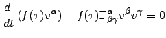
The fortran routine called LSoda which is part of the ODEPACK [1] collection of solvers. One thing to note is that the equation 1 would be more useful written in a way as to allow the differentiation to be done with respect to time. To that end we re-write in the following form,

$$\frac{d\,}{dt}\left(f(\tau)\frac{dx^\alpha}{dt}\right) + f(\... ...alpha_{\beta \gamma}\frac{dx^\beta}{dt}\frac{dx^\gamma}{dt}=0$$ (2)

where,

$$f(\tau)=\frac{dt}{d\tau}$$ (3)

Furthermore, because it is a first order ode solver our equations of motion it will have to be re-written in the first order form,

$$v^\alpha= \frac{dx^\alpha}{dt}$$ (4)

$$\frac{d\,}{dt}\left(f(\tau)v^\alpha \right) + f(\tau)\Gamma^\alpha_{\beta \gamma}v^\beta v^\gamma =0$$ (5)

This doubles the amount of equations we must solve but that will not pose any additional complications. Utilizing a high order Runge-Kutta-Fehlberg method it solves the first order system of ode's. The Runge-Kutta-Fehlberg 4th/5th method is an adaptive stepsize algorithm. It will adjust the stepsize in a way as to keep the fractional error less than the Relative Tol and the absolute error less than Absolute Tol. Relative Tol and Absolute Tol are input parameters in the fortran routine.

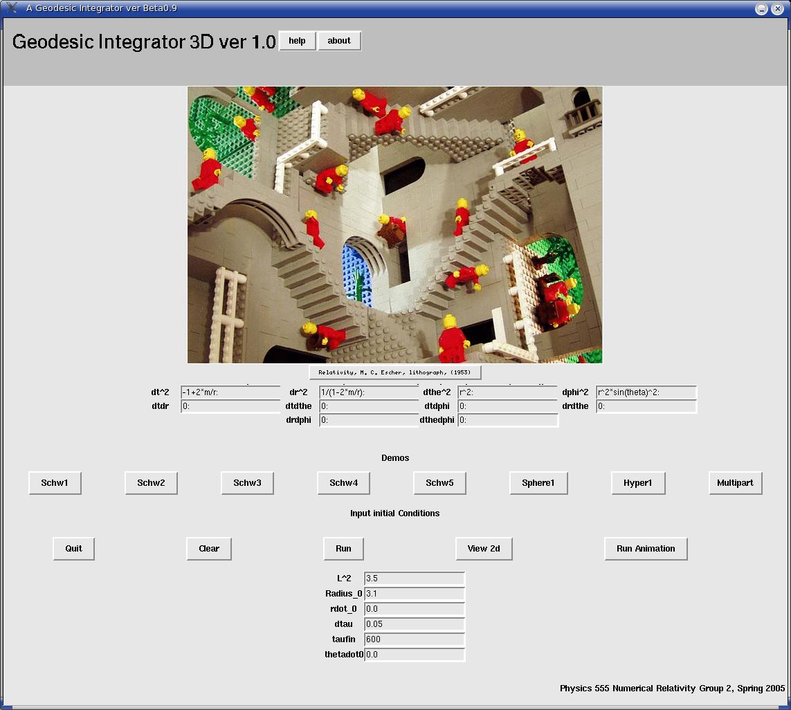
The data is then output in a way that can be understood by xfpp3d. A visualization software that is written in openGL and requires ASCII input. Thus far we have found it to be the best way to render graphics such as ours and has no problem handling dust clouds composed of thousands of individual non-interaction particles. A diagram for the single particle procedure is shown in diagram 2.

Figure 1: GUI Frontend

Figure 2: Architecture

Figure 3: GUI description