next up previous contents
Next: The Routine Up: Visualtization Project: Geodesic Integrator Previous: Introduction and Motivation   Contents

Geodesic Equations

In terms of local coordinates on a given space-time (M) the geodesic equation can be written as [5,6,3]
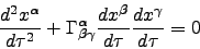
\begin{displaymath}
\frac{d^2 x^\alpha}{d\tau^2} + \Gamma^\alpha_{\beta \gamma}\frac{dx^\beta}{d\tau}\frac{dx^\gamma}{d\tau}=0
\end{displaymath} (1)

The gamma symbols are of course the Christoffel connections or symbols which are, as we know, derivatives of the metric function. For that reason we will need to have access to the derivatives of the metric components. We can use a numerical differentiation but we have chosen to use maple to do this. Maple is used only to find the derivatives and then a fortran routine is used to solve the non-linear differential equations. The fortran routine is much more efficient at handling this than maple especially considering that for a simulation with dust many many operations will take place. In the first assignment we solved this for the special case of the Schwarzschild space-time in a place and we would like to extend this to more general situations. 
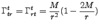
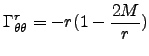
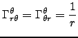
The non-zero Christoffel symbols for Schwarzschild. We calculated them using Maple and GRTensor:


$\displaystyle \Gamma^t_{tr}=\Gamma^t_{rt}=\frac{M}{r^2}(1-\frac{2M}{r})$ $\textstyle \Gamma^r_{tt}=\frac{M}{r^2}(1-\frac{2M}{r})$ $\displaystyle \Gamma^r_{rr}=-\frac{M}{r^2}(1-\frac{2M}{r})$  
$\displaystyle \Gamma^r_{\theta\theta}=-r(1-\frac{2M}{r})$ $\textstyle \Gamma^r_{\phi\phi}=-r sin^2(\theta)(1-\frac{2M}{r})$ $\displaystyle \Gamma^\theta_{r\theta}=\Gamma^\theta_{\theta r}=\frac{1}{r}$  
$\displaystyle \Gamma^\theta_{\phi\phi}=-sin(\theta)cos(\theta)$ $\textstyle \Gamma^\phi_{r\theta}=\Gamma^\phi_{\theta r}=\frac{1}{r}$ $\displaystyle \Gamma^\phi_{\theta\phi}=\Gamma^\phi_{\phi\theta}=cot(\theta)$  

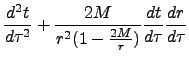
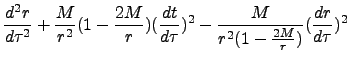
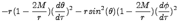
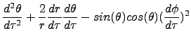
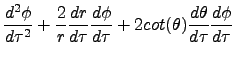
(1) which turns into the following four equations, using spherical coordinates where $\tau$ is an affine parameter1:

$\displaystyle \frac{d^2t}{d\tau^2}+\frac{2M}{r^2(1-\frac{2M}{r})}\frac{dt}{d\tau}\frac{dr}{d\tau}$ $\textstyle =$ $\displaystyle 0$  
$\displaystyle \frac{d^2r}{d\tau^2}+\frac{M}{r^2}(1-\frac{2M}{r})(\frac{dt}{d\tau})^{2}-\frac{M}{r^2(1-\frac{2M}{r})}
(\frac{dr}{d\tau})^2$      
$\displaystyle -r(1-\frac{2M}{r})(\frac{d\theta}{d\tau})^2-rsin^2(\theta)(1-\frac{2M}{r})(\frac{d\phi}{d\tau})^2$ $\textstyle =$ $\displaystyle 0$  
$\displaystyle \frac{d^2\theta}{d\tau^2}+\frac{2}{r}\frac{dr}{d\tau}\frac{d\theta}{d\tau}-sin(\theta)cos(\theta)(\frac{d\phi}{d\tau})^2$ $\textstyle =$ $\displaystyle 0$  
$\displaystyle \frac{d^2\phi}{d\tau^2}+\frac{2}{r}\frac{dr}{d\tau}\frac{d\phi}{d\tau}+2cot(\theta)\frac{d\theta}{d\tau}\frac{d\phi}{d\tau}$ $\textstyle =$ $\displaystyle 0$  


next up previous contents
Next: The Routine Up: Visualtization Project: Geodesic Integrator Previous: Introduction and Motivation   Contents
Benjamin Gutierrez 2005-07-24