Implementation

We wrote a fortran 77 code orbit.f to implement the geodesic integration. We used the routine LSODA which belongs to the ODEPACK package, that we have been using since Physics 410. The LSODA solver was written in Fortran by Alan Hindmarsh and Linda Petzhold of Lawrence Livermore National Labs and is part of the ODEPACK collection of solvers. It is a very robust adaptive stepsize solver that automatically switches to a BDF multistep method if necessary (see the ODEPACK website [2] for more info).

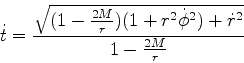
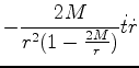
We will simplify the geodesics equations (6) obtained in the preceeding section restricting the motion of our massive particle to the plane $\theta=\pi/2$. In addition, we need to cast our equations in first order form, so they have a suitable form to be integrated by the LSODA routine. Introducing the variables $\dot{t},\dot{r}$ and $\dot{\phi}$ we accomplish this task (where the dot indicates derivative with respect to $\tau$),

$$\frac{dt}{d\tau} = \dot{t}$$

$$\frac{d\dot{t}}{d\tau} = -\frac{2M}{r^2(1-\frac{2M}{r})}\dot{t}\dot{r}$$

$$\frac{dr}{d\tau} = \dot{r}$$

$$\frac{d\dot{r}}{d\tau} = -\frac{M}{r^2}(1-\frac{2M}{r})\dot{t}^2+\frac{M}{r^2(1-\frac{2M}{r})} \dot{r}^2+r(1-\frac{2M}{r})\dot{\phi}^2$$

$$\frac{d\phi}{d\tau} = \dot{\phi}$$

$$\frac{d\dot{\phi}}{d\tau} = -\frac{2}{r}\dot{r}\dot{\phi}$$

The initial conditions for our geodesic paths are choosen to be the following: the initial radius $r$, the initial radial velocity $\dot{r}$, and the square of the angular momentum (per unit mass for a massive particle), $L^2$. We calculate the initial angular velocity using the equation $L=r^2\dot{\phi}$, so $\dot{\phi}_0 = \sqrt{L_2}/{r_0}^2$. The initial condition for $\dot{t}$ is calculated using the metric components in the following way (for a timelike geodesic)

$$\dot{t}_0 = \sqrt{(1+g_{22}{\dot{r}_0}^2+g_{44}{\dot{\phi}_0}^2)/(-g_{11})}$$ (19)

which in our case is

$$\dot{t}=\frac{\sqrt{(1-\frac{2M}{r})(1+r^2\dot{\phi}^2)+\dot{r}^2}}{1-\frac{2M}{r}}$$ (20)

Given the intial conditions we discussed, the program has the following command line input:

orbit <L2> <R0> <Rdot0> <dtau> <tau_f>

The output data will be visualized in two ways: a two-dimensional graph plotted by gnuplot and and the data will also be output in a format suitable for pp2d or xfpp3d (we include a few screenshots of animations).

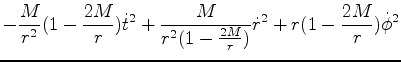
We also coded the subroutine fcn in two ways: the first implementation incorporated the equations of motion in first order form as we saw in (19), and we also used a maple procedure to output the Christoffel symbols as a fortran 77 subroutine. We included the subroutine cg0 in our code and then we coded a general form of the geodesic equations:

$$y'(1) = u\hspace{11.5cm}$$

$$y'(2) = -(\Gamma^{1}_{11}u^2 + \Gamma^{1}_{22}v^2 +\Gamma^{1}_{33}*w^2 +\Gamma^{1}_{44}z^2$$

$$+ 2*\Gamma^{1}_{12}uv+2\Gamma^{1}_{13}uw+2\Gamma^{1}_{14}uz + 2\Gamma^{1}_{23}vw \nonumber$$

$$+2\Gamma^{1}_{24}vz+2*\Gamma^{1}_{34}wz)$$

$$y'(3) = v\hspace{11.5cm}$$

$$y'(4) = -(\Gamma^{2}_{11}u^2 + \Gamma^{2}_{22}v^2+\Gamma^{2}_{33}w^2 +\Gamma^{2}_{44}z^2$$

$$+ 2\Gamma^{2}_{12}uv+2\Gamma^{2}_{13}uw +2\Gamma^{2}_{14}uz + 2\Gamma^{2}_{23}vw$$

$$+2\Gamma^{2}_{24}vz+2\Gamma^{2}_{34}wz)$$

$$y'(5) = z\hspace{11.5cm}$$

$$y'(6) = -(\Gamma^{3}_{11}u^2 + \Gamma^{3}_{22}v^2 +\Gamma^{3}_{33}w^2+\Gamma^{3}_{44}z^2$$

$$+ 2\Gamma^{3}_{12}uv+2\Gamma^{3}_{13}uw+2\Gamma^{3}_{14}uz + 2\Gamma^{3}_{23}vw$$

$$+2\Gamma^{3}_{24}vz+2\Gamma^{3}_{34}wz)$$

A more general form will be used in our term project to be able to plot geodesics in 3D.

The code also produces error messages when the integrator crashes, which occurs when the particle gets close to the eventhorizon or the origin (the geodesic equations become singular of course). The gnuplot script also uses grep and awk to filter messages from usefull data. We leave the mass of the particle, $M$, as a parameter declared in our fcn subroutine.

Finally, to monitor the stability of the solution we calculate the constans of motion of the geodesic , the square of the angular momentum and the energy:

$$E=\dot{t}(1-\frac{2M}{r})$$ (21)

What we do is calculate these conserved quantities at the begining of the numerical experiment, from the initial state. Then we continue calculating them and comparing to the original values and we report the maximum error at the end. We set the LSODA tolerance to $10^{-10}$, and a typical experiment reported errors of the order of:

lnx1 87> orbit 4.0 2.0 0.0 0.01 30
 Integration completed successfully.

 Conserved quantities:
 E =
    1.000000000000000
 maxError E =
   2.2056483306442942E-009
 L2 =
    4.000000000000000
 maxErrorL2 =
   6.4374858776972133E-009

Larger tolerances produce errors in LSODA. So we sticked to this tolerance for most of the experiments. We are aware that some orbits must be more sensitive to this parameter than others, but variating the tolerance did not seem to modify the orbits in any significant way.