The problem that we consider is the one-dimensional wave equation:
where we have adopted the common subscript notation for partial differentiation, and we have set the speed of wave propagation to unity. The general solution of this equation represents a superposition of left moving (l) and right moving (r) waves (radiation):
We will solve the equation on the domain {x = [0..1] : t = [0..T]} with so-called "outgoing radiation" or "Sommerfeld" conditions specified at x = 0 and x = 1. That is, at x = 0 and x = 1, we demand that there be no radiation coming from the left or right respectively. Thus we have
and
We recast the wave equation in first order form (first order in time, first order in space), by introducing auxiliary variables, pp and pi, which are the spatial and temporal derivatives, respectively, of phi:
The wave equation then becomes the following pair of first order equations
and the boundary conditions are
The RNPL code w1dcn_rnpl, solves the above system of equations using a second-order Crank-Nicholson approximation: second-order centred approximations to the spatial derivatives are used for the interior equations, while second-order forward and backward formulas are used for the spatial derivatives needed in the implementation of the left and right boundary conditions respectively. (See the finite difference NOTES, particularly section 1.4.2 for a discussion of Crank-Nicholson schemes).
Hopefully, by this time you will have had a look at the available RNPL documentation, and will be thus be able to understand most of the details of the source code. if you have any questions concerning the implementation, ask one of the lab instructors for assistance.
A tar-ed and gzip-ed distribution for the RNPL solution of the above wave equation is available for download HERE. Download the distribution to some convenient location within your home directory on the lab machines, then upack it via
% tar xzf w1dcn.tar.gzChange to the w1dcn directory and generate a listing of the files therein. You should see the following
% cd w1dcn
% ls
Makefile  id0  id1  id2  id3  id4  w1dcn_rnpl
Build the application by typing make; the make command should generate the following output.
% make
/usr/local/bin/rnpl -l allf  w1dcn_rnpl
rnpl_fix_f77 updates.f initializers.f residuals.f
f77 -O6 -c w1dcn.f
f77 -O6 -c updates.f
f77 -O6 -c residuals.f
f77 -O6 -L/usr/local/lib w1dcn.o updates.o residuals.o -lrnpl -lvs -lsv -o w1dcn
f77 -O6 -c w1dcn_init.f
f77 -O6 -c initializers.f
f77 -O6 -L/usr/local/lib w1dcn_init.o updates.o residuals.o initializers.o -lrnpl -lvs -lsv -o w1dcn_init
Note that the rnpl compilation generates a number of Fortran source files (with .f extensions) and include files (source code fragments with .inc extensions)
% ls *.f *.inc
gfuni0.inc   initializers.f  residuals.f    updates.f  w1dcn_init.f
globals.inc  other_glbs.inc  sys_param.inc  w1dcn.f
as well as two executables, w1dcn, which performs the evolution of the FD system, and w1dcn_init, which generates the intial data for the evolution:
% ls w1dcn w1dcn_init
w1dcn*  w1dcn_init*
If you are so inclined, you may wish to quickly inspect the contents of initializers.f, residuals.f and updates.f.
% w1dcn id0
 Can't open in0.sdf
 Calling initial data generator.
 WARNING: using default for parameter epsiterid.
 WARNING: using default for parameter maxstep.
 WARNING: using default for parameter maxstepid.
 WARNING: using default for parameter s_step.
 WARNING: using default for parameter ser.
 WARNING: using default for parameter start_t.
 WARNING: using default for parameter trace.
 Starting evolution.  step:  0 at t=  0.
 step:  1 t=  0.0125 steps= 7
 step:  2 t=  0.025 steps= 7
 step:  3 t=  0.0375 steps= 6
 step:  6 t=  0.075 steps= 7
            .
            .
            .
 step:  123 t=  1.5375 steps= 11
 step:  124 t=  1.55 steps= 11
 step:  125 t=  1.5625 steps= 11
 step:  126 t=  1.575 steps= 11
 step:  127 t=  1.5875 steps= 11
 step:  128 t=  1.6 steps= 11
The various diagnostic messages written to the terminal require some explanation.
First,
Can't open in0.sdf
Calling initial data generator.
indicates that the intial state file, in0.sdf, that is specified in the parameter file id0 does not exist in the current directory, and thus the initial data generator, w1dcn_init, is automatically invoked to prepare it. w1dcn_init is passed the same parameter file used in the invocation of w1dcn, and then goes about its job of generating the initial state file. Once w1dcn_init has completed this task, w1dcn resumes execution.
During the initialization phases of both w1dcn_init and w1dcn, warning messages are issued if default parameter values are being used for any of the generic RNPL parameters (generic in the sense that they are defined for all RNPL applications). Thus, in the diagnostics, we see the sequence
WARNING: using default for parameter epsiterid.
WARNING: using default for parameter maxstep.
WARNING: using default for parameter maxstepid.
WARNING: using default for parameter s_step.
WARNING: using default for parameter ser.
WARNING: using default for parameter start_t.
WARNING: using default for parameter trace.
appearing twice, first from the execution of w1dcn_init, then from the execution of w1dcn. These particular messages can be safely ignored.
The final sequence of messages:
Starting evolution.  step:  0 at t=  0.
step:  1 t=  0.0125 steps= 7
step:  2 t=  0.025 steps= 7
step:  3 t=  0.0375 steps= 6
step:  6 t=  0.075 steps= 7
			.
			.
			.
step:  123 t=  1.5375 steps= 11
step:  124 t=  1.55 steps= 11
step:  125 t=  1.5625 steps= 11
step:  126 t=  1.575 steps= 11
step:  127 t=  1.5875 steps= 11
step:  128 t=  1.6 steps= 11
represents a trace of the time-stepping alogorithm of the application. The time steps at which diagnostic output, such as
step: 1 t= 0.0125 steps= 7is produced, coincide with the those at which grid function output to .sdf files is generated. Both are controlled by the output parameter, which in id0 is set via
output := 0-*indicating that output (at level 0) is to occur at every time step. In addition to the step number and physical time, the steps = ... diagnostic shows the number of sub-iterations that were required to achieve convergence of the difference equations at that particular time step. The convergence criterion is controlled by the parameter epsiter, which is set in id0 via
epsiter := 1.0e-5
% ls *_0.sdf
pi_0.sdf  pp_0.sdf
one for each of the grid functions for which output has been enabled in the RNPL source code via the {out_gf = 1} directive:
float pp on g1 at 0,1 {out_gf = 1}
float pi on g1 at 0,1 {out_gf = 1}
The sdfinfo command can be used to get summary information about the
contents of an .sdf file:
but more typically, and as discussed briefly below, the data stored in an .sdf file is sent to a visualization utility, such as xvs or DV for inspection and/or analysis.
Start xvs from the command line as follows:
% xvs &
xvs: Starting service on port 5001

xvs: For help/documentation see

http://laplace.physics.ubc.ca/Doc/xvs/
(your invocation of the command will use a different port number)
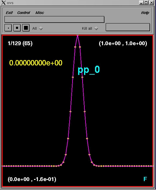
Once xvs is running, you can transmit data to it from 1-D .sdf files using the sdftoxvs command. For example, if you invoke
% sdftoxvs pp_0.sdfor, equivalently
% sdftoxvs pp_0the xvs interface should then look like this:
% diff id0 id1
8c8
< level := 0
---
> level := 1
13,14c13,14
< in_file  := "in0.sdf"
< out_file := "out0.sdf"
---
> in_file  := "in1.sdf"
> out_file := "out1.sdf"
In particular, all 5 id files define the same solution domain and initial data parameters. By running w1dcn with each of the parameter files, we generate a sequence of approximate solutions to the same continuum problem, but with grid resolutions of h (level 0), h/2, h/4, h/8 and h/16. For higher-level runs (i.e. with level other than 0), the RNPL code automatically adjusts the frequency of output so that identical physical output times result from each run. For example, performing a level-1 run, we see
% w1dcn id1
 Can't open in1.sdf
 Calling initial data generator.
 WARNING: using default for parameter epsiterid.
 WARNING: using default for parameter maxstep.
 WARNING: using default for parameter maxstepid.
 WARNING: using default for parameter s_step.
 WARNING: using default for parameter ser.
 WARNING: using default for parameter start_t.
 WARNING: using default for parameter trace.
 WARNING: using default for parameter epsiterid.
 WARNING: using default for parameter maxstep.
 WARNING: using default for parameter maxstepid.
 WARNING: using default for parameter s_step.
 WARNING: using default for parameter ser.
 WARNING: using default for parameter start_t.
 WARNING: using default for parameter trace.
 Starting evolution.  step:  0 at t=  0.
 step:  2 t=  0.0125 steps= 5
 step:  4 t=  0.025 steps= 5
 step:  6 t=  0.0375 steps= 5
 step:  8 t=  0.05 steps= 5
 step:  10 t=  0.0625 steps= 5
 step:  12 t=  0.075 steps= 5
             .
             .
             .
 step:  246 t=  1.5375 steps= 10
 step:  248 t=  1.55 steps= 11
 step:  250 t=  1.5625 steps= 11
 step:  252 t=  1.575 steps= 11
 step:  254 t=  1.5875 steps= 11
 step:  256 t=  1.6 steps= 10
Note that output (both diagnostic and .sdf) is now generated every
two steps, but that the physical output times are commensurate with those
from the level-0 run.
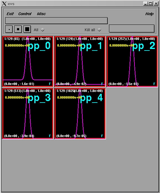
We can quickly perform a series of runs at levels 0 through 4 (output supressed)
% w1dcn id0
% w1dcn id1
% w1dcn id2
% w1dcn id3
% w1dcn id4
then send all of the data for pp to xvs
% xvs ka  Closes pre-existing xvs windows
% sdftoxvs pp_*.sdf
The xvs display should now look like this:
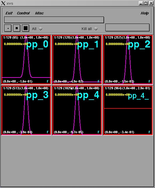
Bring the window labelled pp_4_ to the foreground by positioning the
cursor in it and hitting the space bar. Type S, then use the
right and left mouse buttons to step forward and backward, respectively,
through the results of the convergence test. For example, stepping to the
28th frame, you should see
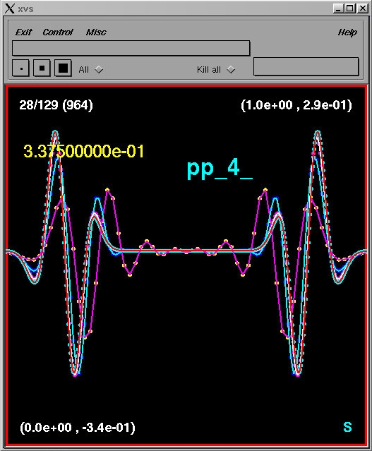
       pp_1 - pp_0
  4 * (pp_2 - pp_1)
 16 * (pp_3 - pp_2)
 64 * (pp_4 - pp_3)
If the results from w1dcn are second-order accurate, then the four
curves should (roughly) coincide, with better and better agreement as the
resolution increases (i.e. for those curves with a higher density of markers).
This is precisely what we see, and this test thus provides a very strong indication
that the code is second-order convergent. (In order to establish that
convergence is to a solution of the original PDE, we could use the technique of
independent residual evaluation; see section 1.9 of the notes on Basic Finite
Difference Techniques for an explanation).
IMPORTANT FINAL NOTE!
Due to the fact that RNPL evolutions always start from an initial state file (such as in0.sdf), one must be very careful that the state file that is read by the application actually corresponds to the desired run parameters. It is a common error to run an RNPL program with the wrong initial state file, and, unfortunately, if can sometimes be difficult to detect that this has happened.
You should get in the habit of always removing the initial state file before running an RNPL code, and you may wish to consider defining a shell alias or script to combine the operations of removing the state file and running the RNPL program.