Next: Implementation of the code
Up: Simple stellar models and
Previous: Simple stellar models and
Contents
The TOV equations
Static, spherically symmetric perfect fluid models in general relativity,
and thus models of stars, are described by the Tolman-Oppenheimer-Volkoff
equation.
The equations for a TOV star [4,5] are usually
given in Schwarzschild coordinates. For a textbook discussion see
Chapter (6.2) in the book by Wald [6].
The notation for the fluid quantities follows [7].
Here we are assuming a perfect fluid matter model, i.e. that the stress energy tensor is given by
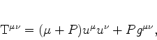 |
(22) |
where  is the total energy,
  the pressure and
  is the fluid
four velocity.
Regarding equations of state, we will focus on the simple family of
polytropic equations of state. Polytropes are self-gravitating gaseous
spheres that are very usefull as a crude approximation of more
realistic stellar models in astrophysics and one can go far using it. More realistic
models incorporate diverse equations of state, for nuclear matter for
example, or quark-gluon plasma state, etc.
is the fluid
four velocity.
Regarding equations of state, we will focus on the simple family of
polytropic equations of state. Polytropes are self-gravitating gaseous
spheres that are very usefull as a crude approximation of more
realistic stellar models in astrophysics and one can go far using it. More realistic
models incorporate diverse equations of state, for nuclear matter for
example, or quark-gluon plasma state, etc.
 |
(23) |
Where  is the rest-mass density .
for
is the rest-mass density .
for  corresponds to an adiabatic star supported by
pressure of non-relativistic gas, and the
corresponds to an adiabatic star supported by
pressure of non-relativistic gas, and the  case
corresponds to an adiabatic star supported by pressure of
ultra-relativistic gas.
case
corresponds to an adiabatic star supported by pressure of
ultra-relativistic gas.
The metric in Schwarzschild coordinates is given by
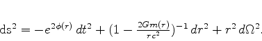 |
(24) |
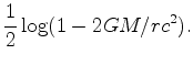
Here  is the gravitational mass inside the sphere of radius
  , and
, and
 is the logarithm of the lapse and can also be interpreted as the
Newtonian gravitational potential.
is the logarithm of the lapse and can also be interpreted as the
Newtonian gravitational potential.
In the exterior vacuum region we have
This allows us to match at the surface of the
star. Note that for numerical hydrodynamical evolutions, the pressure is often
set to a small nonzero value ('atmosphere')
in the exterior for technical reasons.
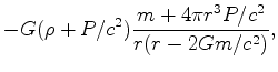
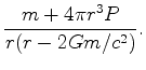
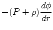
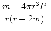
The Einstein equations then imply the TOV system of ODEs (for a derivation
see e.g. [6] or go ahead and try yourself whenever you have time):
Note that the last equation decouples from the first two!
The initial data at  is (for
the numerical integration)
is (for
the numerical integration)
 ,
,  ,
,
 . Note that the equation is singular at , this may require
some attention in the numerical code!
. Note that the equation is singular at , this may require
some attention in the numerical code!
We will choose geometric units where  4.
Rewriting our metric and our equations in geometric units we have,
4.
Rewriting our metric and our equations in geometric units we have,
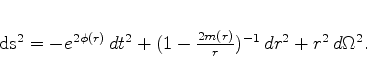 |
(31) |
acts as a relativistic analog of the newtonian
gravitational potential. So the equations we are going to use to
describe the hydrostatic equilibrium inside our compact object is,
where  and
and  are the total energy density and pressure
of the fluid star, respectively. These quantities are measured in the
rest frame.
are the total energy density and pressure
of the fluid star, respectively. These quantities are measured in the
rest frame.
An equivalent form of the TOV equations is obtained substituting
(35) into (34),
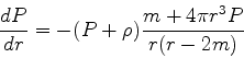 |
(35) |
as we saw before.
Next: Implementation of the code
Up: Simple stellar models and
Previous: Simple stellar models and
Contents
Benjamin Gutierrez
2005-07-23